gwdet
Detectability of gravitational-wave signals from compact binary coalescences
This is a short python module to compute the probability of detecting a gravitational-wave signal from compact binaries averaging over sky-location and source inclination.
The detectability function is defined by Finn and Chernoff in arxiv:9301003 as a function of the projection parameter Theta (their Eq. 3.31). Here however, we follow the notation of Dominik+ in arxiv:1405.7016, which defined w= Theta/4 such that 0<=w<=1. We are interested in the cumulative distribution P(>w) of the projection parameter w (see their Eq. A.1). This gives the probabilty that an elliptically polarized gravitational-wave signal (like that of a binary) will be detected taking into account the antenna pattern of the detector and the inclination of the source (here we consider a single detector, even if in the real world we deal with networks…).
For a given (non-spinning) compact binary with masses m1 and m2 at redshift z, you first need to compute its signal-to-noise ratio snr_opt assuming optimal orientation and location (i.e. the source is face on, overhead the detector). Then specify a threshold, say 8, above which you consider the signal detectable. The probabilty that a specific binary will be detected is just P(w=8/snr_opt).
Right now this code can only handle non-spinning systems. I will generalize it to spinning sources, eventually (any help is very welcome! Send a me a pull request).
Cite me…
If you use this software in a scientific publication, I kindly ask you to cite its DOI:
This code is developed and maintained by Davide Gerosa. To report bugs, please open an issue on GitHub. If you want to contact me, it’s dgerosa@caltech.edu.
Results
gwdet has been used in the following papers:
- Taylor and Gerosa (2018) arXiv:1808.02491
- Gerosa et al. (2018) arXiv:1808.02491
Installation and checkpoints
You can install this module using pip
pip install gwdet
Dependancies include numpy, scipy,matplotlib,astropy,requests and pathos will be installed automatically if not present. The LIGO software lal and pycbc are needed to use this code with values other than the default ones (see here for a short guide I wrote).
If you limit yourself to the default values, I provide some checkpoints files which let you use the code without installing any LIGO software. In any case, even if you have lal, dowloading these checkpoints will save you a lot of computational time. When you use the code with defaults parameters for the first time, a message like the following will be printed out:
[gwdet] You are using defaults values. You can download this interpolant. Use:
    curl ....
To download the checkpoints, just execute that whole command starting with curl. There are two checkpoint files of ~5MB and ~200MB. Note that these files will not be removed if you uninstall the module via pip uninstall , you will need to remove them manually. If you install gwdet in a virtual environment, these checkpoint files will live in the environment directory and will be removed when/if you delete the environment.
Usage
This code has two classes only, averageangles and detectability. You first need to create an instance of each class and then use them.
The default usage is
p=gwdet.averageangles()
w=0.5 # Projection parameter
print(p(w)) # Fraction of detectabile sources

p=gwdet.detectability()
m1=10. # Component mass in Msun
m2=10. # Component mass in Msun
z=0.1  # Redshift
print(p(m1,m2,z))  # Fraction of detectabile sources
averageangles
Compute the detection probability, averaged over all angles (sky location, polarization, inclination, etc), as a function of the projection parameter w.
p = averageangles(  directory=os.path.dirname(__file__),
                binfile=None,
                mcn=int(1e8),
                mcbins=int(1e5) )

det = p(w) # with 0<=w<=1
Parameters:
directory: where checkpoints are stored (default is the module location)binfile: checkpoint file (ifNonecomputed from other kwargs)mcn: resolution parameter (number of Monte Carlo samples)mcbins: resolution parameter (number of interpolated bins)w: projection parameter 0<=w<=1, see arxiv:1405.7016 (can be float or array)
Returns:
det: GW detectability (float or array)
detectability
Compute the detection probability of a non-spinning compact binary.
p = detectability(  directory=os.path.dirname(__file__),
                binfile=None,
                binfilepdet=None,
                approximant='IMRPhenomD',
                psd='aLIGOZeroDetHighPower',
                psd_from_path=False,
                psd_path=None,
                is_asd_file=None,
                flow=10.,
                deltaf=1./40.,
                snrthreshold=8.,
                massmin=1.,
                massmax=100.,
                zmin=1e-4,
                zmax=2.2,
                mc1d=int(200),
                mcn=int(1e8),
                mcbins=int(1e5),
                parallel=True,
                screen=False)

det = p(m1,m2,z)
Parameters:
directory: where checkpoints are stored (default is the module location)binfile: checkpoint file (if None computed from other kwargs)binfilepdet: checkpoint file (if None computed from other kwargs)approximant: waveform appriximant used to compute SNRs. Available list:pycbc.waveform.waveform.print_fd_approximants()psd: power spectral density used to compute SNRs. Available list:pycbc.psd.analytical.get_lalsim_psd_list()psd_from_path: load psd usingpycbc.psd.from_txt(default False)psd_path: power spectral density used to compute SNRs. Provide path to.txtfile (default None)is_asd_file: check whether thetxtfile contains amplitude or power spectral density (default True)flow: starting frequency in SNR calculationsdeltaf: resolution parameter (frequency sampling)snrthreshold: minimum detectable signalmassmin,massax: limits on the component masses in Msun. Interpolated inside, extrapolated outsidezmin,zmax: limits on the redshift. Interpolated inside, extrapolated outsidemc1d: resolution parameter (number of grid point per dimension)mcn: resolution parameter (number of Monte Carlo samples)mcbins: resolution parameter (number of interpolated bins)parallel: use parallel jobs on all CPUs availablescreen: debug option, prints all SNRs computedm1: component mass in Msun (can be float or array)m2: component mass in Msun (can be float or array)z: redshift (can be float or array)
Returns:
det: GW detectability (float or array)
Checks and performance
Here I first compare the performance of the P(w) interpolator implemented in averageangles against public data from Emanuele Berti’s website. The agreement is excellent and the residuals are just numerical noise. This plot can be generated with:
gwdet.compare_Pw()

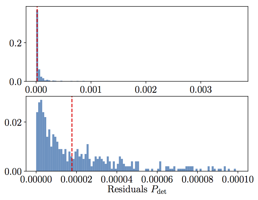
Seconly, I compare the perfomance of the P(m1,m2,z) interpolator of detectability against 1000 bruce force SNR computations from lal. Altough occasional mismathces of 3% are found, the median residuals are as small as ~1e-5. This plot can be generated with:
gwdet.compare_Psnr()
