Examples
This is a short
notebook
to illustrate some of the key features of the precession module.
There much more than this in the code but hopefully this is a good
starting point.
>>> import numpy as np
>>> from importlib.machinery import SourceFileLoader
>>> precession = SourceFileLoader("precession", "../precession/precession.py").load_module()
>>> precession_eccentricity = SourceFileLoader("eccentricity", "../precession/eccentricity.py").load_module()
The import syntax above ensures that the online documentation grabs the
latest version. For you, it should just be import precession for the
main code that deals with quasi-circular binaries. If you’re using the
eccentric version, we reccommend importing with
import precession.eccentricity as precession.
1. Select a binary configuration.
First, set the constants of motion. These include mass ratio and spin magnitudes:
>>> q = 0.8
>>> q
0.8
>>> chi1 = 0.5
>>> chi1
0.5
>>> chi2 = 0.9
>>> chi2
0.9
From these, find a suitable value of the effective spin within its geometrical limits
>>> chieff_minus,chieff_plus=precession.chiefflimits(q=q, chi1=chi1, chi2=chi2)
>>> chieff = 0.1
>>> assert chieff>=chieff_minus and chieff<=chieff_plus
>>> chieff
0.1
Now the quantities that vary on the radiation-reaction timescale. Specify the orbital separation
>>> r = 1000
>>> r
1000
Find a suitable value of the asymptotic angular momentum (its boundaries are the spin-orbit resonances):
>>> kappa_minus,kappa_plus=precession.kappalimits(r=r,chieff=chieff, q=q, chi1=chi1, chi2=chi2)
>>> kappa = 0.02
>>> assert kappa>=kappa_minus and kappa<=kappa_plus
This is more conventiently done by specifying a dimensionless number, e.g.
>>> kappa = precession.kapparescaling(kappatilde=0.5, r=r, chieff=chieff, q=q, chi1=chi1, chi2=chi2)
>>> kappa
array([0.04563644])
Finally, the precession-timescale variation is encoded in the weighted spin difference. Its limits are given by the solutions of a cubic polynomial:
>>> deltachi_minus,deltachi_plus = precession.deltachilimits(kappa=kappa,r=r,chieff=chieff,q=q,chi1=chi1,chi2=chi2)
>>> deltachi=-0.1
>>> assert deltachi>=deltachi_minus and deltachi<=deltachi_plus
You can also sample deltachi from its PN-weighted porability density function
>>> deltachi = precession.deltachisampling(kappa=kappa, r=r, chieff=chieff, q=q, chi1=chi1, chi2=chi1, N=1)
Or, as before, specify a dimensionless number, e.g.
>>> deltachi = precession.deltachirescaling(deltachitilde=0.4, kappa=kappa, r=r, chieff=chieff, q=q, chi1=chi1, chi2=chi2)
>>> deltachi
array([-0.15027382])
From these quantities, one can compute the spin angles
>>> theta1, theta2, deltaphi = precession.conserved_to_angles(deltachi=deltachi, kappa=kappa, r=r, chieff=chieff, q=q, chi1=chi1, chi2=chi2)
>>> theta1,theta2,deltaphi
(array([1.66141316]), array([1.25261228]), array([1.4089439]))
The inverse operation is
>>> deltachi_, kappa_, chieff_ = precession.angles_to_conserved(theta1=theta1, theta2=theta2, deltaphi=deltaphi, r=r, q=q, chi1=chi1, chi2=chi2)
>>> assert np.isclose(deltachi_,deltachi) and np.isclose(kappa_,kappa) and np.isclose(chieff_,chieff)
One can now compute various derived quantities including:
The precession period
The total precession angle
Two flavors of the precession estimator chip
The spin morphology
… and many more!
>>> tau = precession.eval_tau(kappa=kappa, r=r, chieff=chieff, q=q, chi1=chi1, chi2=chi2)
>>> tau
array([1.14179292e+09])
>>> alpha = precession.eval_alpha(kappa=kappa, r=r, chieff=chieff, q=q, chi1=chi1, chi2=chi2)
>>> alpha
array([34.7076951])
>>> chip_averaged = precession.eval_chip(deltachi=deltachi,kappa=kappa,r=r,chieff=chieff,q=q,chi1=chi1,chi2=chi2,which="averaged")
>>> chip_averaged
array([0.74912589])
>>> chip_rms = precession.eval_chip(deltachi=deltachi,kappa=kappa,r=r,chieff=chieff,q=q,chi1=chi1,chi2=chi2,which="rms")
>>> chip_rms
array([0.81485269])
>>> morph = precession.morphology(kappa=kappa, r=r, chieff=chieff, q=q, chi1=chi1, chi2=chi2 )
>>> morph
array(['C+'], dtype='<U32')
2. Inspiral
Let’s now evolve that binary configuration down to r=10M.
>>> rvals = [r, 10] # Specify all the outputs you want here
>>> outputs = precession.inspiral_precav(kappa=kappa,r=rvals,chieff=chieff,q=q,chi1=chi1,chi2=chi2)
>>> outputs
{np.str_('theta1'): array([[1.55654632, 1.61559444]]),
 np.str_('theta2'): array([[1.32832283, 1.28585682]]),
 np.str_('deltaphi'): array([[ 2.53842303, -1.82082625]]),
 np.str_('deltachi'): array([[-0.0920836 , -0.12487951]]),
 np.str_('kappa'): array([[0.04563644, 0.06977371]]),
 np.str_('r'): array([[1000,   10]]),
 np.str_('u'): array([[0.06403612, 0.64036123]]),
 np.str_('deltachiminus'): array([[-0.19622919, -0.42562113]]),
 np.str_('deltachiplus'): array([[-0.08134075,  0.26825594]]),
 np.str_('deltachi3'): array([[0.74325701, 0.1801658 ]]),
 np.str_('chieff'): array([0.1]),
 np.str_('q'): array([0.8]),
 np.str_('chi1'): array([0.5]),
 np.str_('chi2'): array([0.9])}
The same evolution can also be done with an orbit-averaged scheme (note that now you have to specify deltachi as well). This is slow:
>>> outputs = precession.inspiral_orbav(deltachi=deltachi, kappa=kappa,r=rvals,chieff=chieff,q=q,chi1=chi1,chi2=chi2)
>>> outputs
{np.str_('t'): array([[0.000000e+00, 7.935974e+10]]),
 np.str_('theta1'): array([[1.66141316, 0.88395959]]),
 np.str_('theta2'): array([[1.25261228, 1.76230812]]),
 np.str_('deltaphi'): array([[1.4089439, 3.0730197]]),
 np.str_('Lh'): array([[ 0.03131792,  0.        ,  0.99950947],
        [ 0.00124545, -0.06643326,  0.99779009]]),
 np.str_('S1h'): array([[-0.73494006,  0.67476338, -0.06750919],
        [ 0.1569422 , -0.79776378,  0.58218745]]),
 np.str_('S2h'): array([[-0.73753054, -0.5857321 ,  0.33610506],
        [-0.13214016,  0.98330163, -0.12513137]]),
 np.str_('deltachi'): array([[-0.15027382,  0.25227467]]),
 np.str_('kappa'): array([[0.04563644, 0.06865318]]),
 np.str_('r'): array([[1000,   10]]),
 np.str_('u'): array([[0.06403612, 0.64036123]]),
 np.str_('chieff'): array([[0.1       , 0.09999999]]),
 np.str_('q'): array([0.8]),
 np.str_('chi1'): array([0.5]),
 np.str_('chi2'): array([0.9]),
 np.str_('cyclesign'): array([[1., 1.]])}
Let’s now take this binary at r=10M, and propagate it back to past time infinity:
>>> rvals = [outputs['r'][0,-1], np.inf] # Specify all the outputs you want here
>>> outputs = precession.inspiral_precav(kappa=outputs['kappa'][0,-1],r=rvals,chieff=chieff,q=q,chi1=chi1,chi2=chi2)
>>> outputs
{np.str_('theta1'): array([[2.10290286, 1.66496015]]),
 np.str_('theta2'): array([[0.92438427, 1.25002889]]),
 np.str_('deltaphi'): array([[0.89512712, 1.57212042]]),
 np.str_('deltachi'): array([[-0.38186097, -0.15223596]]),
 np.str_('kappa'): array([[0.06865318, 0.04154245]]),
 np.str_('r'): array([[10., inf]]),
 np.str_('u'): array([[0.64036123, 0.        ]]),
 np.str_('deltachiminus'): array([[-0.43153997, -0.15223596]]),
 np.str_('deltachiplus'): array([[ 0.25313088, -0.15223596]]),
 np.str_('deltachi3'): array([[0.18034069,        nan]]),
 np.str_('chieff'): array([0.1]),
 np.str_('q'): array([0.8]),
 np.str_('chi1'): array([0.5]),
 np.str_('chi2'): array([0.9])}
3. Precession average what you like
The code also allow you to precession-average quantities specified by the users. For instance, let’s compute the average of deltachi.
>>> def func(deltachi):
...     return deltachi
...
>>> deltachiav_ = precession.precession_average(kappa=kappa, r=r, chieff=chieff, q=q, chi1=chi1, chi2=chi2, func=func)
>>> deltachiav_
array([-0.13857097])
For this specific case, the averaged can also be done semi-analytically in terms of elliptic integrals (though in general this is not possible). Let’s check we get the same result:
>>> u = precession.eval_u(r, q)
>>> deltachiminus,deltachiplus,deltachi3 = precession.deltachiroots(kappa=kappa, u=u, chieff=chieff, q=q, chi1=chi1, chi2=chi2)
>>> m = precession.elliptic_parameter(kappa=kappa, u=u, chieff=chieff, q=q, chi1=chi1, chi2=chi2,
...                                   precomputedroots=np.stack([deltachiminus, deltachiplus, deltachi3]))
>>> deltachiav = precession.inverseaffine( precession.deltachitildeav(m),  deltachiminus, deltachiplus)
>>> deltachiav
array([-0.13857097])
>>> (deltachiav_-deltachiav)/deltachiav
array([-5.72653799e-13])
This is also an example of how providing the optional quantity
precomputedroots speeds up the computation.
4. Evolution of an eccentric and precessing binary
Note when using the eccentric version of precession: The code is
implemented such that almost all functions available in precession
can be accessed by simply importing its eccentric extension. Some of
them are exactly the same as in the circular counterpart;
others—specifically those directly involving time or orbital
separation—require different inputs (briefly: all r parameters have
been replaced with (a, e)). Functions that are specific to the
circular case only (such as eval_r or those related to remnant
properties) cannot be accessed via precession.eccentricity.
To evolve an eccentric and spin-precessing black hole binary from a larger semi-major axis (which can be thought of as a proxy for the orbital separation) to a smaller one, it is necessary to also state the initial eccentricity along with information about the masses and spins of the system.
>>> #intial semi major axis ( in geometric units)
>>> np.random.seed(42)
>>> a0= 100
>>> #final semi major axis
>>> af= 10
>>> a_array= np.linspace(a0, af, 100) #array of semi-major axis values for the inspiral
>>> #initial eccentricity
>>> e0 = 0.6
>>> #spin parameters
>>> chi1 =np.random.uniform(0.1, 1)
>>> chi2 =np.random.uniform(0.1, 1)
>>> theta1, theta2, deltaphi = precession_eccentricity.isotropic_angles(N=1)
>>> #mass parameters
>>> q = np.random.uniform(0.1, 1)
>>> output_ecc=precession_eccentricity.inspiral_precav(theta1=theta1,theta2=theta2,deltaphi=deltaphi,a=a_array,e=e0,q=q,chi1=chi1,chi2=chi2)
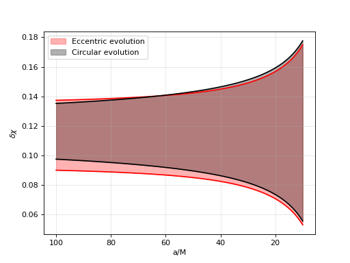
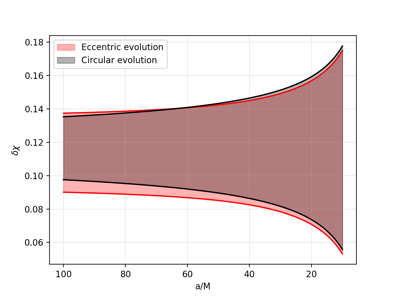
Let’s compare it with a circular evolution (setting e=0)
>>> output_circ=precession_eccentricity.inspiral_precav(theta1=theta1,theta2=theta2,deltaphi=deltaphi,a=a_array,e=0,q=q,chi1=chi1,chi2=chi2)
The spin angles evolve differently!
>>> import pylab as plt
>>>
>>>
>>> plt.plot(output_ecc['a'][0], output_ecc['deltachiminus'][0],color='red')
>>> plt.plot(output_ecc['a'][0], output_ecc['deltachiplus'][0], color='red')
>>> plt.plot(output_circ['a'][0], output_circ['deltachiminus'][0],color='k')
>>> plt.plot(output_circ['a'][0], output_circ['deltachiplus'][0],color='k')
>>>
>>>
>>> plt.fill_between(
...     output_ecc['a'][0],
...     output_ecc['deltachiminus'][0],
...     output_ecc['deltachiplus'][0],
...     color='red',
...     alpha=0.3,
...     label='Eccentric evolution'
>>> )
>>>
>>>
>>> plt.fill_between(
...     output_circ['a'][0],
...     output_circ['deltachiminus'][0],
...     output_circ['deltachiplus'][0],
...     color='k',
...     alpha=0.3,
...     label='Circular evolution'
>>> )
>>>
>>> plt.xlabel('a/M')
>>> plt.ylabel('$\delta \chi$')
>>> plt.legend()
>>> plt.grid(True, alpha=0.3)
>>> plt.gca().invert_xaxis()
>>> plt.show()
>>>
Matplotlib is building the font cache; this may take a moment.